
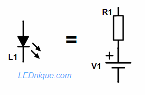
LEDs do not have a linear relationship between current and voltage so they cannot be modeled as simply as a resistor using Ohm’s Law, \( V = IR \). We can, however, make a simplification and model them over a range of currents as a combination of a resistor and a voltage source.
If we look at a typical LED IV curve we can see that it is approximately linear over much of its useful range. This allows us to model the LED as a resistor and voltage source.
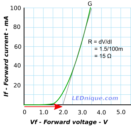
In Figure 1 the grey line is reasonably close to the LED curve from 20 mA to 100 mA. We can work out the resistance that this represents from Ohm’s law \( V = IR \) but in this case we will look at the change in voltage and current in the area of interes.
\( R = \frac{\Delta V}{\Delta I} = \frac{3.5 – 2.0}{100m – 0} = \frac{1.5}{100m} = 15 \mathrm\Omega \).
We can also see that the line crosses the X-axis at Vf = 2.0 V. Our equivalent circuit for this region of interest is (referring to Figure 2) R1 = 15 Ω and V1 = 2.0 V.
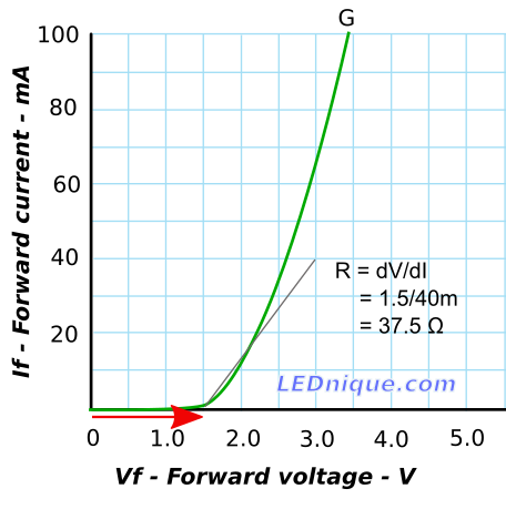
If we are interested in the lower current range of the LED, 1 to 20 mA, for example, we can calculate again. In this case the ends of the grey line have differences of 1.5 V and 40 mA giving a slope of 37.5 Ω. The voltage source becomes 1.5 V.